Tutorials

Loop over all spectra in SMASS

To loop over all spectra in a given source, use the Spectra class.

smass = classy.Spectra(source = "SMASS") # select all asteroids based on source

for spec in smass:
    print(spec.target.name, spec.target.number)

Loop over all spectra in classy index

To loop over all spectra in your classy index, you can load the index and pass it to Spectra. As the index can be quite large, it’s recommended to do this in chunks.

idx = classy.index.load() # returns classy index as pd.DataFrame

# Load spectra in chunks of 100
N = 10

for i in range(0, len(idx), N):
    specs = classy.Spectra(idx.iloc[i:i+N])

You can set skip_target=True to skip target resolution via rocks and significantly speed up the process.

for i in range(0, len(idx), N):
    specs = classy.Spectra(idx.iloc[i:i+N], skip_target=True)

Excluding points based on SNR or flag values

To exclude a reflectance value from the classification, you can set it to NaN.

import numpy as np

import classy

# Get Gaia spectrum of Ceres
ceres = classy.Spectra(1, source="Gaia")  # returns classy.Spectra instance

# "ceres" is now a list of classy.Spectrum entries which only one element, the Gaia spectrum
# We simplify by removing the list and getting the first entry
ceres = ceres[0]  # returns classy.Spectrum instance

# Classify and plot the result
ceres.classify()
ceres.plot(taxonomy='mahlke')

# There are sketchy data points
# Exclude points where the flag is not 0
ceres.refl[ceres.flag != 0] = np.nan

# Exclude the last point
ceres.refl[-1] = np.nan

# Preprocess, classify and plot again
ceres.classify()
ceres.plot(taxonomy='mahlke')

From spectrum to classification

This tutorial shows how to collect and combine spectra of a single asteroid, perform some tasks, and classifying the spectra in different taxonomic schemes.

We start with imports and gathering the spectra of our target (1685) Toro from online repositories.

import classy

import pandas as pd

# ------
# Get spectra from online repositories
spectra = classy.Spectra("toro")

Next, we add our own spectrum of (1685) Toro to the list of remote spectra.

# ------
# Add my own observation
data = pd.read_csv(
    "my_toro_spectrum.csv",
    names=["wavelength", "reflectance", "uncertainty", "flag"],
    skiprows=1,
)

my_spec = classy.Spectrum(
    # mandatory
    wave=data["wavelength"],
    refl=data["reflectance"],
    # optional but used by classy
    refl_err=data["uncertainty"],
    flag=data["flag"],
    source="OBSZ2",
    name="toro",
    # optional and ignored by classy
    date_obs="2022/02/19",
    phase_angle=23,
)

# Add my spectrum to the literature ones
spectra = spectra + my_spec

An extract of my_toro_spec.csv looks like this:

wave,refl,unc,flag
0.4350,0.8798,0.0099,0
0.4375,0.8674,0.0090,0
0.4400,0.8682,0.0082,0
0.4425,0.8842,0.0075,0
0.4450,0.8672,0.0068,0
        [...]
2.4300,1.4123,0.0102,0
2.4350,1.4169,0.0103,0
2.4400,1.4095,0.0103,0
2.4450,1.4158,0.0105,0
2.4500,1.4178,0.0105,0

Let’s see what we data we have now.

# ------
# Print some information
print(f"There are {len(spectra)} spectra of (1685) Toro:")

for spec in spectra:
    # for the literature spectra
    if spec.source != "OBSZ2":
        # Print the source and reference
        source_shortbib = f"{spec.source} / {spec.shortbib}"
    # for my spectrum
    else:
        source_shortbib = "My Observation"

    # Add the covered wavelength range and the number of datapoints
    waverange = f"{spec.wave.min():.2f} - {spec.wave.max():.2f}µm"
    N = f"N={len(spec)}"

    print(
        f"  {source_shortbib:<33}{waverange:<15}{N}",
    )

This prints:

There are 10 spectra of (1685) Toro:
  Gaia / Galluccio+ 2022           0.37 - 1.03µm  N=16
  SMASS / Burbine and Binzel 2002  0.88 - 1.64µm  N=42
  SMASS / Binzel+ 2004             0.43 - 2.43µm  N=492
  MITHNEOS / Binzel+ 2019          0.43 - 2.48µm  N=531
  MITHNEOS / Binzel+ 2019          0.82 - 2.48µm  N=320
  MITHNEOS / Binzel+ 2019          0.43 - 2.45µm  N=523
  MITHNEOS / Binzel+ 2019          0.43 - 2.48µm  N=541
  MITHNEOS / Binzel+ 2019          0.43 - 2.48µm  N=572
  MITHNEOS / Binzel+ 2019          0.43 - 2.43µm  N=501
  My Observation                   0.43 - 2.45µm  N=493

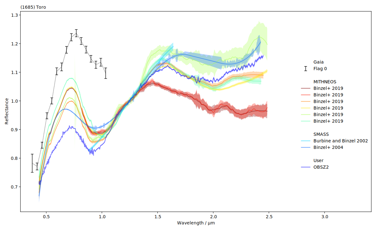
We can inspect them visually as well. classy shows the reflectance values and, if provided, the uncertainty as a shaded region around the spectrum.

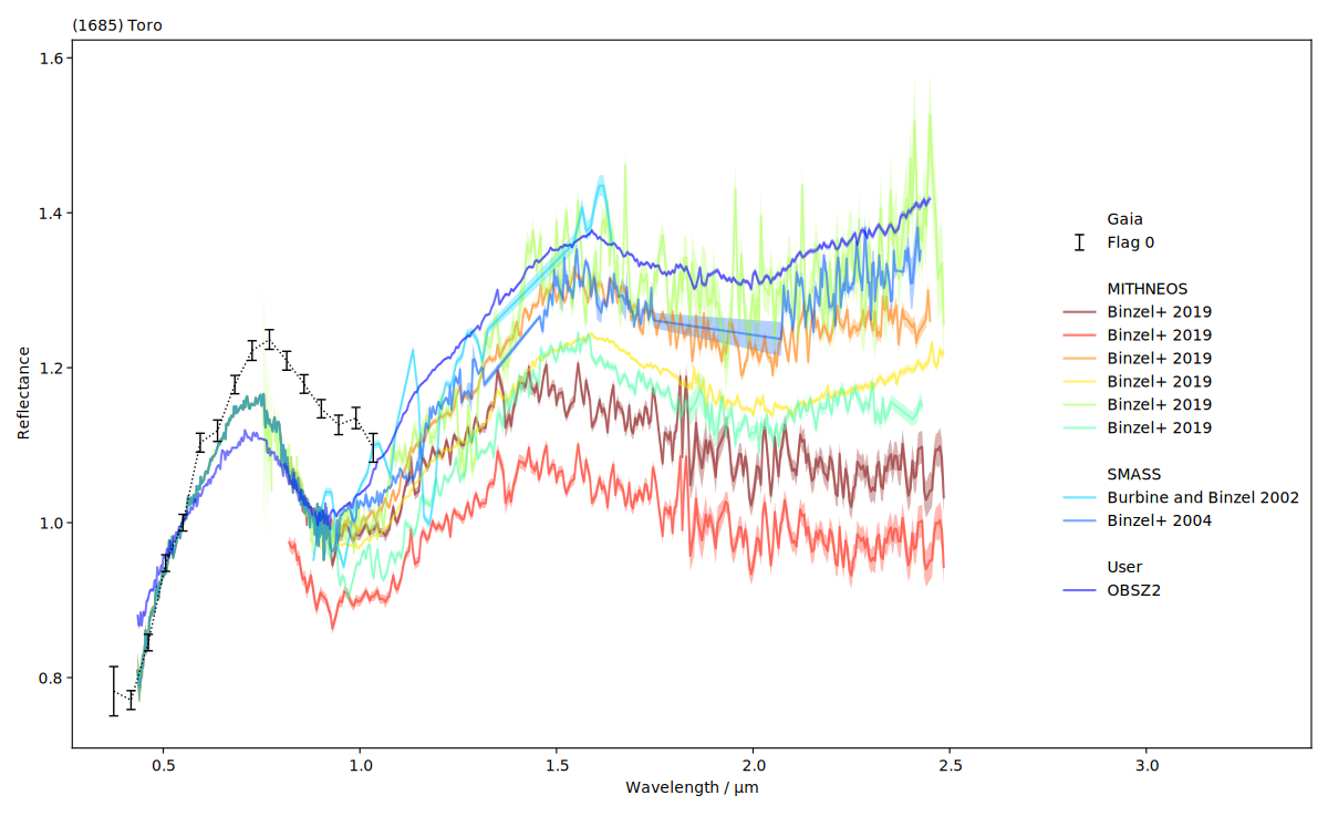
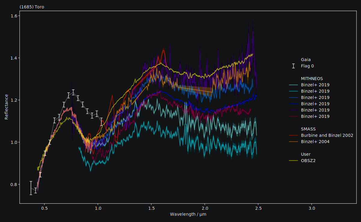
We see that the SMASS and MITHNEOS spectra are densely sampled yet noisy. We can apply different smoothing techniques in a simple for-loop.

# ------
# Apply smoothing with specific parameters for each spectrum
for spec in spectra:
    if spec.source == "MITHNEOS":
        spec.smooth(method="savgol", window_length=int(len(spec) / 10), polyorder=3)
    elif spec.source == "SMASS":
        spec.smooth(method="spline", k=3, s=0.5)

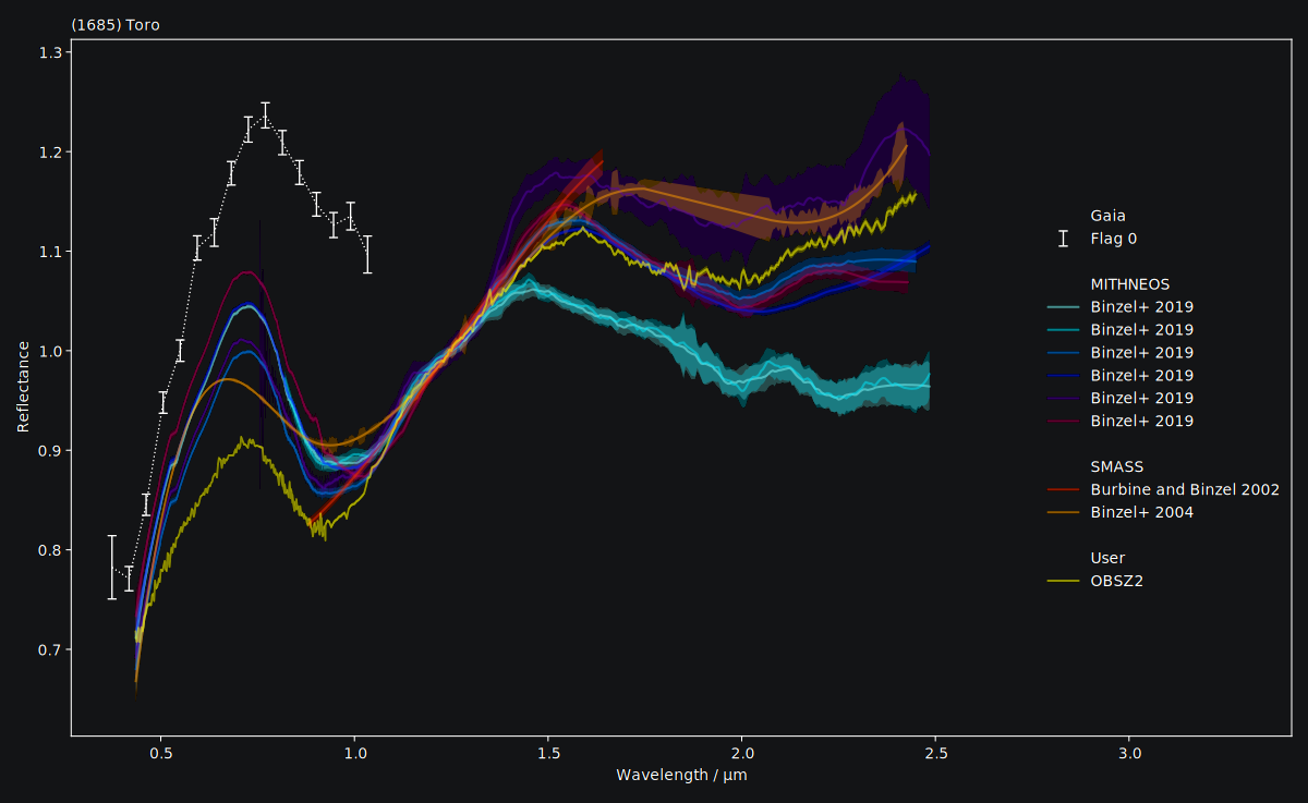
Again, we can visually inspect the result.

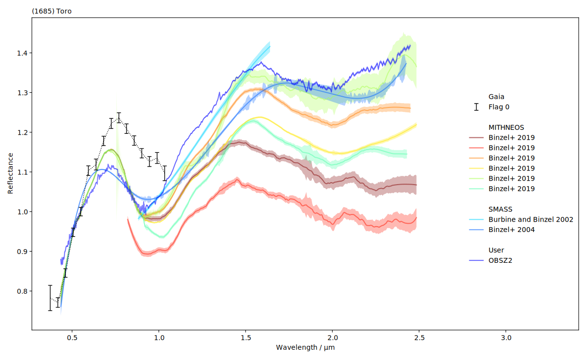
It could be easier to visually compare the spectra if they had the same normalisation.

# ------
# Normalize to 1.25µm if this wavelength was observed
wave_norm = 1.25

for spec in spectra:
    if spec.wave.min() < wave_norm <= spec.wave.max():
        spec.normalize(at=wave_norm)

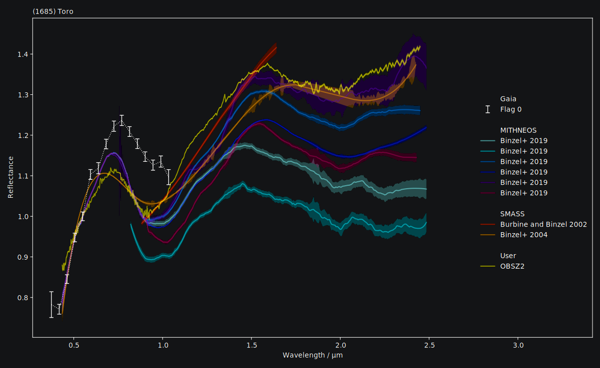
# Inspect the result
spectra.plot()

Now we get to classifying the spectra. Note that classy will automatically apply the necessary normalisations and wavelength grids required for each taxonomy to the reflectance spectra prior to classification, and revert the changes after classifying.

# ------
# Classify spectra in possible schemes
for spec in spectra:
    spec.classify()  # taxonomy='mahlke' is default
    spec.classify(taxonomy="demeo")
    spec.classify(taxonomy="tholen")

Now we can inspect the classes. If the required wavelength range for the Tholen 1984 and DeMeo+ 2009 taxonomies are not covered (and the taxonomies cannot be applied), the corresponding attributes are simply empty strings.

# print the classification results
for spec in spectra:
    # for the literature spectra
    if spec.source != "OBSZ2":
        # Print the source and reference
        source_shortbib = f"{spec.source} / {spec.shortbib}"
    # for my spectrum
    else:
        source_shortbib = "My Observation"

    # Add the covered wavelength range and the number of datapoints
    waverange = f"{spec.wave.min():.2f} - {spec.wave.max():.2f}µm"
    N = f"N={len(spec)}"

    print(
        f"  {source_shortbib:<33}{waverange:<15}{N:<5} T84: {spec.class_tholen:<3}DM09: {spec.class_demeo:<4}M22:{spec.class_:<2}({spec.prob*100:.1f}%)",
    )

This prints:

Gaia / Galluccio+ 2022           0.37 - 1.03µm  N=16  T84: S  DM09:     M22:S (90.2%)
SMASS / Burbine and Binzel 2002  0.88 - 1.64µm  N=42  T84:    DM09:     M22:S (99.9%)
SMASS / Binzel+ 2004             0.43 - 2.43µm  N=492 T84:    DM09:     M22:S (98.8%)
MITHNEOS / Binzel+ 2019          0.43 - 2.48µm  N=531 T84:    DM09: S   M22:Q (52.6%)
MITHNEOS / Binzel+ 2019          0.82 - 2.48µm  N=320 T84:    DM09:     M22:S (65.5%)
MITHNEOS / Binzel+ 2019          0.43 - 2.45µm  N=523 T84:    DM09: Sqw M22:S (98.7%)
MITHNEOS / Binzel+ 2019          0.43 - 2.48µm  N=541 T84:    DM09: Sqw M22:Q (52.7%)
MITHNEOS / Binzel+ 2019          0.43 - 2.48µm  N=572 T84:    DM09: Sqw M22:S (97.0%)
MITHNEOS / Binzel+ 2019          0.43 - 2.43µm  N=501 T84:    DM09:     M22:Q (77.5%)
My Observation                   0.43 - 2.45µm  N=493 T84:    DM09: Sqw M22:S (99.9%)

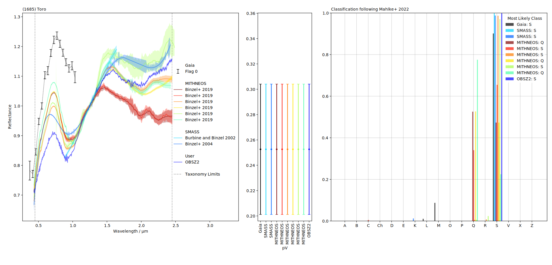
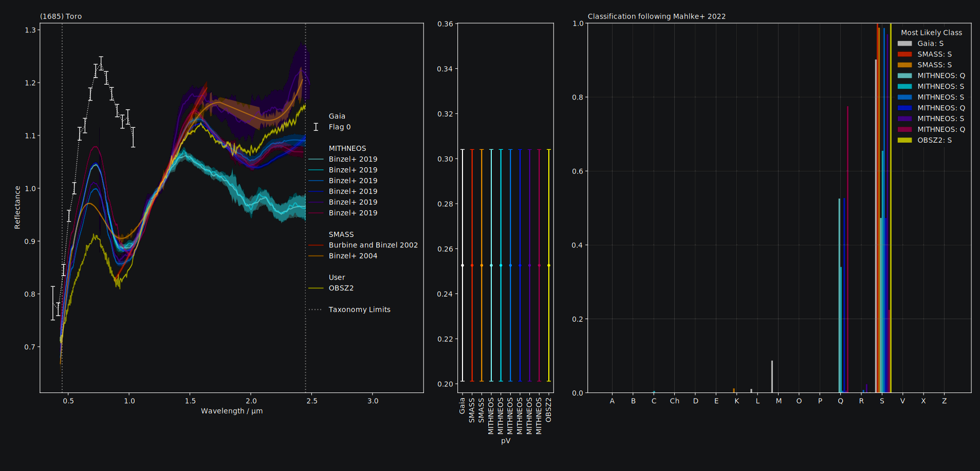
We can inspect the classification result in a plot:

spectra.plot(taxonomy='mahlke')  # taxonomy='mahlke' is default

Duplicating a Spectrum

To compare different preprocessing strategies, it might be useful to create a copy of an existing Spectrum. Use the python built-in function copy.deepcopy() for this.

>>> import classy
>>> import copy
>>> baucis = classy.Spectra(172, source='SMASS')[0]  # returns classy.Spectrum
>>> baucis_copy = copy.deepcopy(baucis)  # create identical copy
>>> baucis_copy.smooth()  # smooth only the copy
>>> spectra = baucis + baucis_copy  # returns classy.Spectra
>>> spectra.plot()  # compare