Classifying Spectra

classy can taxonomically classify asteroid spectra and return the classification results as well as visualize them. Classification results might be more reliable after preprocessing the spectra and identifying features relevant for the class assignment. All tasks can be done via the command line interface and the python interface.

Command Line

Classify all available spectra of (21) Lutetia.

$ classy classify lutetia
+---------+--------+----------+----------+--------+--------------+-------------+--------------+-------------------------+
| name    | number | wave_min | wave_max | albedo | class_mahlke | class_demeo | class_tholen | shortbib                |
+---------+--------+----------+----------+--------+--------------+-------------+--------------+-------------------------+
| Lutetia | 21     | 0.337    | 1.041    | 0.19   | K            |             | M            | Zellner+ 1985           |
| Lutetia | 21     | 2.515    | 4.997    | 0.19   | S            |             |              | Usui+ 2019              |
| Lutetia | 21     | 0.440    | 2.490    | 0.19   | M            | Xc          |              | Unpublished             |
| Lutetia | 21     | 0.435    | 2.450    | 0.19   | M            | X           | M            | Unpublished             |
| Lutetia | 21     | 0.440    | 2.450    | 0.19   | M            | Xc          |              | Unpublished             |
| Lutetia | 21     | 0.820    | 2.490    | 0.19   | M            |             |              | Ockert-Bell+ 2010       |
| Lutetia | 21     | 0.501    | 0.920    | 0.19   | L            |             |              | Lazzaro+ 2004           |
| Lutetia | 21     | 0.752    | 2.501    | 0.19   | M            |             |              | Hardersen+ 2011         |
| Lutetia | 21     | 0.374    | 1.034    | 0.19   | M            |             | M            | Galluccio+ 2022         |
| Lutetia | 21     | 0.440    | 2.490    | 0.19   | M            | Xc          |              | DeMeo+ 2009             |
| Lutetia | 21     | 0.913    | 2.300    | 0.19   | S            |             |              | Clark+ 1995             |
| Lutetia | 21     | 0.330    | 1.060    | 0.19   | M            |             | M            | Chapman and Gaffey 1979 |
| Lutetia | 21     | 0.435    | 0.925    | 0.19   | K            |             |              | Bus and Binzel 2002     |
| Lutetia | 21     | 0.874    | 1.640    | 0.19   | S            |             |              | Burbine and Binzel 2002 |
| Lutetia | 21     | 0.829    | 2.466    | 0.19   | L            |             |              | Bell+ 1988              |
+---------+--------+----------+----------+--------+--------------+-------------+--------------+-------------------------+
                                                      15 Spectra

By default, this prints a table of available spectra and their classification result.

python

Classify all available spectra of (21) Lutetia.

>>> import classy
>>> spectra = classy.Spectra(21)
>>> spectra.classify()

classy automatically applies the required preprocessing (e.g. normalising, resampling) for the respective taxonomic scheme. This happens “under the hood” and does not change the wave and refl attributes of the Spectrum.

Iterate over the list of spectra to inspect the classification result:

>>> for spec in spectra:
>>>     print(f"Spectrum of {spec.shortbib} is of class {spec.class_}")

For brevity, the outputs of the remaining examples in this section are not shown. After having completed the Getting Started section, all shown commands should run on your machine, and you can follow along by copy-pasting them.

Taxonomy Selection

Asteroids can be classified in different taxonomic schemes. The chosen scheme affects the classification procedure (preprocessing steps and classification logic), the required wavelength range of the spectra, and the classification output. classy takes care of the first point, so only the last two points are relevant for you. You can find an overview of the currently supported taxonomies and their basic properties here. To select the scheme of your choice, use the taxonomy argument.

Taxonomy	Argument Value
Mahlke+ 2022	mahlke
DeMeo+ 2009	demeo
Tholen 1984	tholen

The default value is mahlke.

Command Line

$ classy classify vesta --taxonomy demeo

python

>>> spectra.classify(taxonomy="demeo")

The results of the last classification is stored in class_. In case you use different schemes for comparison, you can access the results using class_mahlke, class_demeo, class_tholen.

>>> spectra.classify(taxonomy="demeo")
>>> spec.class_demeo

If a spectrum cannot be classified in the chosen scheme due to insufficient wavelength coverage, a warning is printed and the resulting class is an empty string "".[1] Classification by-products like principal component scores and class probabilities are also available depending on the chosen taxonomy. The products of each scheme can be found in the relevant sections of the overview.

All implemented schemes benefit from knowing the albedo of the target. For mahlke and tholen, this heavily influences the resulting classification. For demeo, classy uses the albedo to resolve branches of the original decision tree that are unresolved in DeMeo+ 2009, in case the classes are reliably different in albedo (e.g. D and S).

A classy.Spectrum can be classified following different taxonomies using the .classify() function. The taxonomy argument can be used to choose between different taxonomies.

>>> import classy
>>> ceres = classy.Spectra(1, source='Gaia')[0]
>>> ceres.classify() # taxonomy='mahlke' is default
>>> ceres.classify(taxonomy='tholen') # Tholen 1984 (requires extrapolation)
>>> ceres.classify(taxonomy='demeo') # DeMeo+ 2009 (fails due to wavelength range)

The resulting class is added as class_ attribute to the spectrum. For tholen and demeo, the attributes are class_tholen and class_demeo respectively. Further added attributes depending on the chosen taxonomy are described in the taxonomies section.

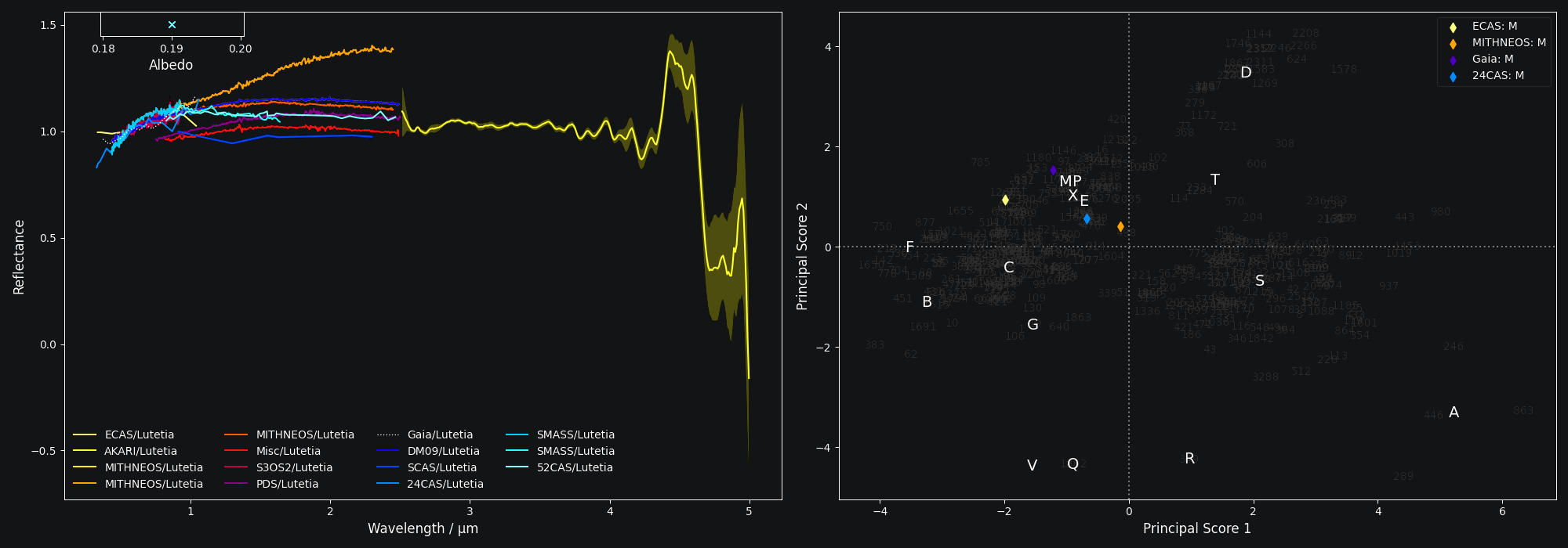
Visualizing the Result

Passing the taxonomy argument to the plot method of the Spectrum and Spectra classes adds a second panel next to the spectra showing the classification result. If taxonomy="mahlke" is set, the results shows the class probabilities for each spectrum.

If taxonomy="demeo" or taxonomy="tholen", it shows the projection of the spectra into the space spanned by the first and second principal components of the respective taxonomies.

>>> spectra = classy.Spectra(21)
>>> spectra.classify(taxonomy='tholen')
>>> spectra.plot(taxonomy='tholen')

On the command line, the classification results can be visualised by specifying the --plot flag. Use the --taxonomy argument to provide the desired taxonomic scheme.

$ classy classify 13 --plot --taxonomy demeo

Exporting the Result

Both Spectrum and Spectra have an export method which can be used to store any of their attributes to a csv file. By default, the Spectrum.export method stores the spectral data (wavelength, reflectance), while the Spectra.export method stores metadata attributes like the classification results, bibliography, or filenames. The usage of the Spectrum.export method is described here.

The Spectra.export method expects a filename as mandatory argument. The attributes to export can be specified using the optional columns argument. By default,[2]

columns = ['name', 'target.name', 'class_mahlke', 'class_demeo', 'class_tholen', 'filename']

Other columns of interest could be the presence of features or their parameters or the class probabilities following the Mahlke taxonomy (see here):

columns = ['target.name', 'class_mahlke', 'class_Q',  'class_S', 'h.is_present', 'h.center', 'shortbib']

Let’s see this in action:

>>> import classy
>>> spectra = classy.Spectra(214)
>>> spectra.classify()
>>> spectra.classify(taxonomy='demeo')
>>> spectra.classify(taxonomy='tholen')
>>> spectra.export('class_aschera.csv')

which gives

$ cat class_aschera.csv
name,target.name,class_mahlke,class_demeo,class_tholen,filename
ECAS/Aschera,Aschera,E,,E,pds/gbo.ast.ecas.phot/data/214.csv
Misc/Aschera,Aschera,E,,,pds/gbo.ast-mb.reddy.spectra/data/2006/214_aschera.tab
S3OS2/Aschera,Aschera,E,,,pds/EAR_A_I0052_8_S3OS2_V1_0/data/n00166_n00307/00214_aschera.tab
Gaia/Aschera,Aschera,E,,E,gaia/part05/aschera.csv
DM09/Aschera,Aschera,E,,E,demeo2009/a000214.sp33.txt
Misc/Aschera,Aschera,E,,,pds/gbo.ast.irtf-spex-collection.spectra/data/clarketal2004/214_030816t055017.tab
SMASS/Aschera,Aschera,S,,,smass/smass2/a000214.[2]

The only practical difference between Spectrum.export and Spectra.export is thus the default value of the columns argument. You can export the the classification results of a single Spectrum by specifying the columns argument:

>>> spec.export("44_nysa_smoothed.csv", columns=["name", "target.name", "class_mahlke", "class_demeo", "class_tholen", "filename"])

To export the spectral data of many Spectra, run the Spectrum.export method in a loop:

>>> for spec in spectra:
...     spec.export(f"{spec.name}.csv")

[1]

If the missing part represents less than a given limit, the spectrum will be extrapolated linearly to cover the required range for classification. This is most useful for the Gaia DR3 spectra (0.374 - 1.034μm) and the Tholen taxonomy (0.337 - 1.041µm). More on this limit and its configuration can be found here.

[2]

The name attribute represents the source of the spectrum and the name of its target, if specified, e.g. Gaia/Lutetia.