Basic Usage

classy is a tool for the analysis of reflectance spectra. Every spectrum is represented the Spectrum class. This class stores the data and metadata of the spectrum and its target. You can build a spectrum in two ways: by providing your own data or by retrieving data from public repositories.

Creating a Spectrum

To create a Spectrum, you require a list of wavelength values and a list of reflectance values:

>>> import classy
>>> # Define dummy data
>>> wave = [0.45, 0.5, 0.55, 0.6, 0.65, 0.7, 0.75, 0.8, 0.85]
>>> refl = [0.85, 0.94, 1.01, 1.05, 1.04, 1.02, 1.04, 1.07, 1.1]
>>> spec = classy.Spectrum(wave=wave, refl=refl)

Let’s have a look at this spectrum.

>>> spec.plot()

The plot legend gives the source and the target name for each spectrum, as explained below. As we have not yet set a target, it is shown as “Unknown”.

Besides the mandatory wave and refl arguments, there are optional arguments with a pre-defined meaning to classy. For example, the refl_err attribute contains the reflectance errors.

>>> refl_err = [0.05, 0.04, 0.03, 0.05, 0.06, 0.03, 0.03, 0.04, 0.07]
>>> spec = classy.Spectrum(wave=wave, refl=refl, refl_err=refl_err)
>>> spec.plot()

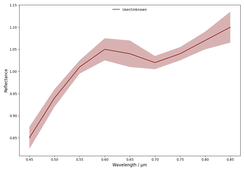
classy automatically adds the error bars to the plot as it recognises the refl_err attribute. You can find a list of all mandatory and optional arguments with a pre-defined meaning for classy below.

Parameter	Accepted values	Explanation
wave	list of float	The wavelength bins of the spectrum in micron.
refl	list of float	The reflectance values of the spectrum.
refl_err	list of float	The uncertainty of the reflectance values of the spectrum.
date_obs	str	Observation epoch of the spectrum in ISOT format: YYYY-MM-DDTHH:MM:SS.
pV	float	The albedo of the target. If not specified but target is set, classy will try to get the albedo from rocks. Relevant for Mahlke/Tholen taxonomies.
phase	float	The phase angle at the epoch of observation in degree.
target	str or int	Name, number, or designation of the asteroidal target of the observation.[1]
source	str	Short string representing the source of the spectrum. Default is ‘User’.

You can specify these when creating the Spectrum or at a later point via the dot-notation. All attributes can be accessed and edited via the dot-notation.

>>> spec.date_obs = '2020-02-01T00:00:00'  # adding metadata to existing spectrum
>>> print(f"Spectrum acquired on {spec.date_obs}.")  # accessing metadata via the dot-notation
Spectrum acquired on 2020-02-01T00:00:00.

Any other arguments you pass to classy.Spectrum or set via the dot-notation are automatically added to the Spectrum, which is useful to define metadata relevant for your analysis, such as flags.[2]

>>> wave = [0.45, 0.5, 0.55, 0.6, 0.65, 0.7, 0.75, 0.8, 0.85]
>>> refl = [0.85, 0.94, 1.01, 1.05, 1.04, 1.02, 1.04, 1.07, 1.1]
>>> flags = [1, 0, 0, 0, 0, 0, 0, 1, 2]
>>> spec = classy.Spectrum(wave=wave, refl=refl, flags=flags)

Assigning a Target

Spectra in classy are typically associated to a minor body. You can specify the target of the observation or setting the target argument when instantiating the Spectrum instance (see table above) or by calling the set_target() method. Both require the name, number, or designation of the target. classy then resolves the target’s identity using rocks and retrieve its physical and dynamical properties, making them accessible via the target attribute. classy makes use of this information in various ways, therefore, it is generally beneficial to specify the target.

>>> spec.set_target('vesta')  # Assigns rocks.Rock instance to spec.target
>>> print(spec.target)
Rock(number=4, name='Vesta')
>>> print(spec.target.number)
4
>>> print(spec.target.albedo.value)
0.380
>>> print(spec.target.class_)
'MB>Inner'

For example, if both the target and the observation date date_obs of a Spectrum are provided, classy can query the phase angle at the time of observation from the Miriade webservice and make it accessible via the phase attribute.

>>> spec.date_obs = '2010-07-01T22:00:00'
>>> spec.compute_phase_angle()
>>> print(f"{spec.target.name} was observed on {spec.date_obs} at a phase angle of {spec.phase:.2f}deg")
Vesta was observed on 2010-07-01T22:00:00 at a phase angle of 23.63deg

Note

classy separates properties of the spectrum and properties of the target. spec.name is the name of the spectrum, spec.target.name is the name of the target. Similarly, properties like the albedo are accessed via the target: spec.target.albedo.value.

Exporting a Spectrum

You can use the export method of the Spectrum class to export the spectral data.

By default, classy will write the current values of the wave, refl, and (if not None) refl_err values to a csv file and save it under the provided path, the mandatory argument of the export function.

>>> spec = classy.Spectra(44, source="Gaia")[0]
>>> spec.export("44_nysa.csv")

A preview of the exported file:

$ head 44_nysa.csv
wave,refl,refl_err
0.374,0.9158446185000001,0.00070279953
0.418,0.941973123,0.0005009585
0.462,0.9665745012000001,0.0004947147
0.506,0.9972719497,0.0005286616
0.55,1.0,0.0005227076
0.594,1.0108662,0.0005877005
0.638,1.001265,0.00057106547
0.682,1.0139798,0.0005213781
0.726,1.0250095,0.0005411855

You can specify which attributes to export by passing a list of attribute names to the columns argument. By default, this list is ['wave', 'refl', 'refl_err']. All attributes must have the same length.

>>> spec.export("44_nysa_with_flag.csv", columns=['wave', 'refl', 'flag'])

$ head 44_nysa_original.csv
wave,refl,flag
0.374,0.9158446185000001,0
0.418,0.941973123,0
0.462,0.9665745012000001,0
0.506,0.9972719497,0
0.55,1.0,0
0.594,1.0108662,0
0.638,1.001265,0
0.682,1.0139798,0
0.726,1.0250095,0

To get the original data of the spectrum, set raw=True. In this case, classy copies the data file of the spectrum from the classy data directory to the specified paths. The columns argument is ignored if raw=True.

>>> spec.export("44_nysa_original.csv", raw=True)

$ head 44_nysa_original.csv
source_id,solution_id,number_mp,denomination,nb_samples,num_of_spectra,refl,refl_err,wave,flag
-4284966856,4167557769573408785,44,nysa,16,21,0.85592955,0.00070279953,0.374,0
-4284966856,4167557769573408785,44,nysa,16,21,0.89711726,0.0005009585,0.418,0
-4284966856,4167557769573408785,44,nysa,16,21,0.94762206,0.0004947147,0.462,0
-4284966856,4167557769573408785,44,nysa,16,21,0.98739797,0.0005286616,0.506,0
-4284966856,4167557769573408785,44,nysa,16,21,1.0,0.0005227076,0.55,0
-4284966856,4167557769573408785,44,nysa,16,21,1.0108662,0.0005877005,0.594,0
-4284966856,4167557769573408785,44,nysa,16,21,1.001265,0.00057106547,0.638,0
-4284966856,4167557769573408785,44,nysa,16,21,1.0139798,0.0005213781,0.682,0
-4284966856,4167557769573408785,44,nysa,16,21,1.0250095,0.0005411855,0.726,0

The export method of the Spectra class behaves differently and is explained later on.

Working with Spectra

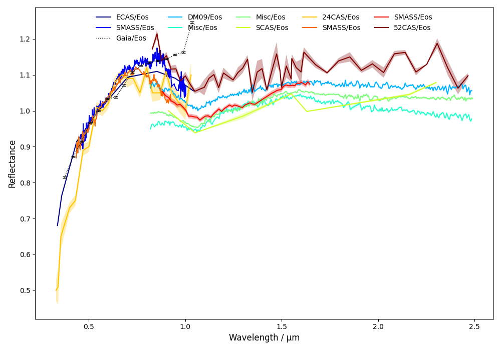
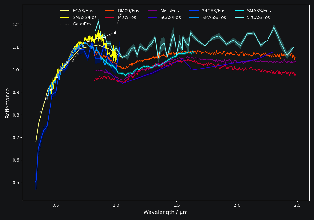
classy is connected to several public repositories of asteroid reflectance spectra. The Spectra class allows to query these repositories for spectra matching a wide range of criteria to ingest them into your analysis (or just to have a look around, which is fun, too). For example, you can query all databases for any spectra of an asteroid by providing its name or number.

>>> spectra = classy.Spectra(221)  # look up spectra of (221) Eos
>>> print(f"Found {len(spectra)} spectra of (221) Eos")
Found 11 spectra of (221) Eos
>>> spectra.plot()

The Spectra class is essentially a list of Spectrum instances. You can the usual python indexing and iteration operations to access the individual spectra.

>>> for spec in spectra:
...     print(f"{spec.source:>6} {spec.shortbib:>15} [{spec.wave.min():.3f}-{spec.wave.max():.3f}]")
 ECAS   Zellner+ 1985 [0.337-1.041]
SMASS        Xu+ 1995 [0.457-1.002]
 Gaia Galluccio+ 2022 [0.374-1.034]
 DM09     DeMeo+ 2009 [0.435-2.485]
 Misc     Clark+ 2009 [0.820-2.485]
 Misc     Clark+ 2009 [0.820-2.490]
 SCAS     Clark+ 1995 [0.913-2.300]
>>> eos_gaia = spectra[2]
>>> print(eos_gaia.shortbib)
Galluccio+ 2022

More examples and advanced query criteria are outlined in the Selecting Spectra chapter.

All literature spectra have their corresponding target assigned automatically.

>>> spectra = classy.Spectra(shortbib="Morate+ 2016")
>>> for spec in spectra[:5]:  # only print 5, Morate+ 2016 observed many more
...     print(spec.target.name)
2001 DC6
2003 YY12
1999 NE28
2000 YZ6
1999 FG51

Besides the attributes of the Spectrum class given in the table above, all public spectra further have the attributes below relating to their bibliography, while additional attributes are available on a per-source basis, as given in the individual repository descriptions.

Attribute	Description
shortbib	Short version of reference of the spectrum.
bibcode	Bibcode of reference publication of the spectrum.
source	String representing the source of the spectrum (e.g. '24CAS').

Dates of Observations

A lot of effort further went into extracting the date_obs parameters of public spectra from the literature and storing them in ISOT format: YYYY-MM-DDTHH:MM:SS. If the literature does not provide the date_obs, it is set to an empty string: "". If the time of the day is not know, HH:MM:SS is set to 00:00:00. If the spectrum is an average of observations at different dates, all dates are given, separated by a ,, e.g. 2004-03-02T00:00:00,2004-05-16T00:00:00.

Phase Angles

Using the dates of observations, classy can query the phase angle of the asteroid at the time of observation. You can do this for all spectra in the classy index using the classy status command, then pressing 1 to manage the cache followed by 2 to add phase angle information to all spectra with known dates of observations. This information is permanently stored in the cache and available via the phase attribute of the Spectrum class.

$ classy status

Contents of /home/mmahlke/astro/data/classy:

    69525 asteroid reflectance spectra from 32 sources [public|private]

    24CAS      285    52CAS      119    AKARI       64    B07         10
    BCU         11    CDS         88    D18         14    DM09       366
    E11         66    EB03        13    ECAS       589    F14        100
    G12         30    Gaia     60518    HARTSS      82    M4AST      123
    MANOS      225    MITHNEOS  1905    Misc       907    P11          7
    P18        146    PDS         91    PRIMASS    437    S08          1
    S3OS2      820    SCAS       126    SMASS     2256    TE12         3
    W17         25    YJ07         5    YJ11        20    dL10        73


Choose one of these actions:
[0] Do nothing [1] Manage cache [2] Retrieve public spectra (0): 1

Choose one of these actions:
[0] Do nothing [1] Rebuild index [2] Add phase angles [3] Clear cache (0): 2

Querying Miriade [=====                                         ] 792 / 7406

Alternatively, for a given Spectrum with a known target and date_obs, you can use the compute_phase_angle() method to query the phase angle.

>>> spec = classy.Spectrum(wave=[0.45, 0.5, 0.55], refl=[0.85, 0.94, 1.01], target="Vesta", date_obs="2024-06-11T07:51:10")
>>> spec.compute_phase_angle()
>>> spec.phase
13.811

Spectrum + Spectra

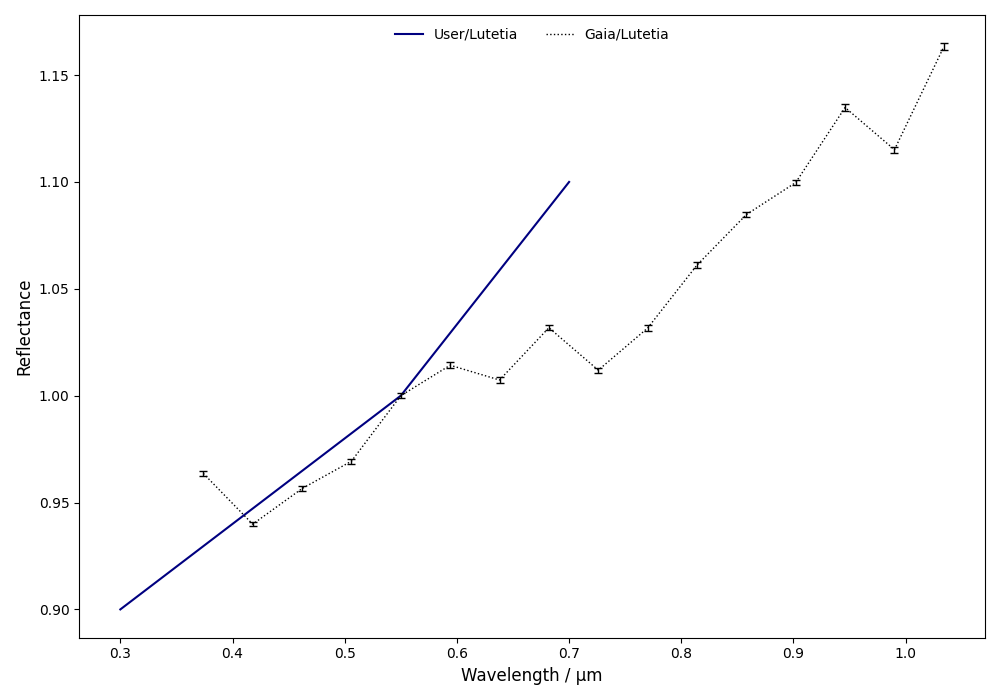
You can combine your observations (Spectrum instances) with observations from the literature (Spectra) by simply adding them.

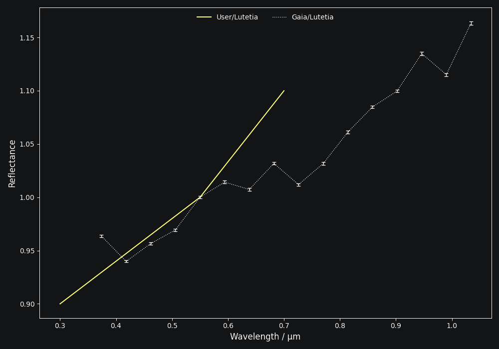
>>> my_lutetia = classy.Spectrum(wave=[0.3, 0.4, 0.55, 0.7], refl=[0.9, 0.94, 1, 1.1], target="Lutetia")
>>> lutetia_literature = classy.Spectra(21, source='Gaia')
>>> lutetia_spectra = my_lutetia + lutetia_literature  # add my_lutetia to the literature results
>>> lutetia_spectra.plot()

The benefit of combining them in a single Spectra instance is that most operations that can be done on a Spectrum (e.g. preprocessing, feature detection, see later chapters) can be done on a large number of Spectra by simply calling the corresponding function of the Spectra class. This saves efforts in typing and is useful when plotting and exporting analysis results.

Plotting Spectra

This chapter already demonstrated taht you can use the plot method of the Spectrum and Spectra classes to visualise the spectra. The method returns the matplotlib Figure and axis instances. If you want to adapt the figure before opening the plot, you can set show=False. This can be useful e.g. if you would like to add template spectra of taxonomic classes for comparison.

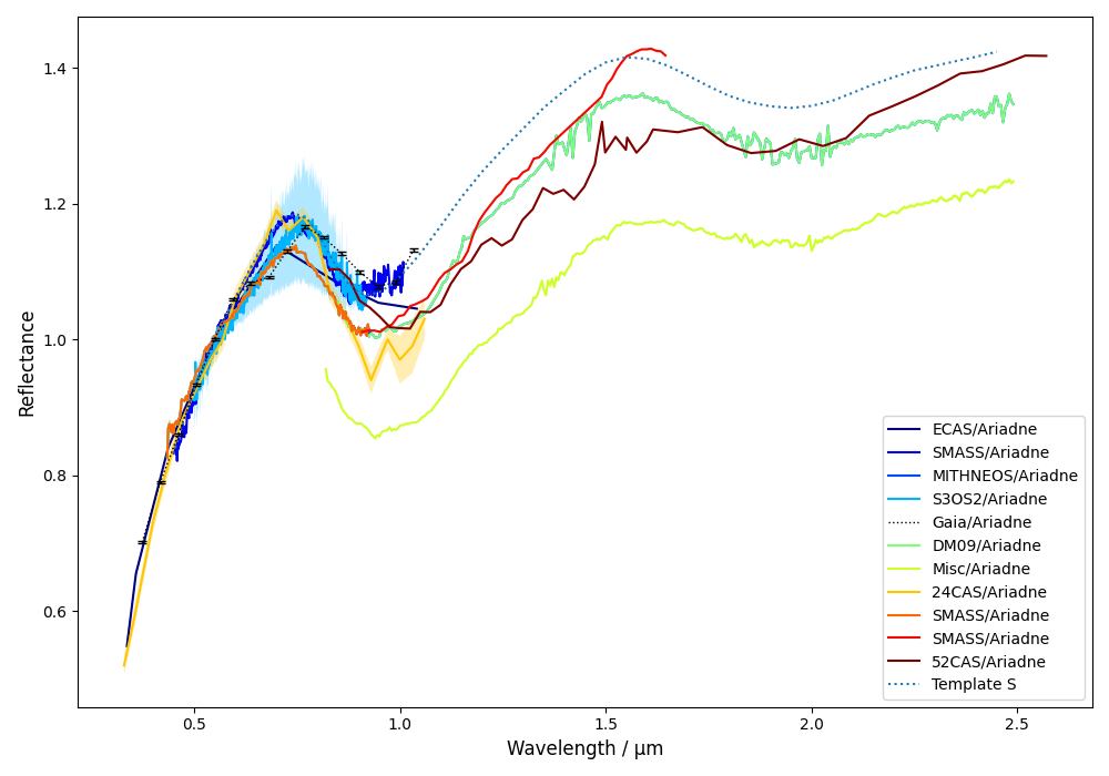
>>> import matplotlib.pyplot as plt
>>> spectra = classy.Spectra(43)
>>> fig, ax = spectra.plot(show=False)
>>> templates = classy.taxonomies.mahlke.load_templates()
>>> ax.plot(templates['S'].wave, templates['S'].refl, label='Template S', ls=":")
>>> ax.legend()
>>> plt.show()

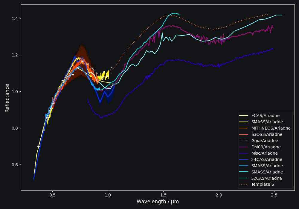
You can save the figure to file by specifying the output filename with the save argument.

>>> spectra.plot(save="43_with_mahlke_s_template.png")

Selecting many Spectra

If you pass a query that matches many spectra to the Spectra class, it can take a while to load all the data and the corresponding target information. If you are primarily interested in the spectra metadata or you would like to refine your search quickly, you can search the classy spectra index with the same syntax. Instead of spectra, this method returns a pandas.DataFrame with the metadata of the matching spectra.

>>> classy.index.query(source="MITHNEOS", wave_min=0.9)
                                       name    source  ... err_phase                          filename
filename                                               ...
mithneos/sp61/a000364.sp61.txt        Isara  MITHNEOS  ...       NaN    mithneos/sp61/a000364.sp61.txt
mithneos/sp68/a000006.sp68.txt         Hebe  MITHNEOS  ...       0.0    mithneos/sp68/a000006.sp68.txt
mithneos/sp75/a000245.sp75.txt         Vera  MITHNEOS  ...       0.0    mithneos/sp75/a000245.sp75.txt
mithneos/sp75/a000079.sp75.txt     Eurynome  MITHNEOS  ...       0.0    mithneos/sp75/a000079.sp75.txt
mithneos/sp92/a000057.sp92.txt    Mnemosyne  MITHNEOS  ...       0.0    mithneos/sp92/a000057.sp92.txt
...                                     ...       ...  ...       ...                               ...
mithneos/dm19/a316934.dm19n1.txt  2001 AA52  MITHNEOS  ...       0.0  mithneos/dm19/a316934.dm19n1.txt
mithneos/dm19/a283319.dm19n2.txt   1992 WR4  MITHNEOS  ...       0.0  mithneos/dm19/a283319.dm19n2.txt
mithneos/dm19/a409995.dm19n1.txt   2006 WV3  MITHNEOS  ...       0.0  mithneos/dm19/a409995.dm19n1.txt
mithneos/dm19/a412976.dm19n2.txt    1987 WC  MITHNEOS  ...       0.0  mithneos/dm19/a412976.dm19n2.txt
mithneos/dm19/a363505.dm19n1.txt  2003 UC20  MITHNEOS  ...       0.0  mithneos/dm19/a363505.dm19n1.txt

[1905 rows x 14 columns]

>>> # that's a lot of specra, let's refine the search
>>> classy.index.query(source='MITHNEOS', wave_min=0.9, family="Themis")
                                   name    source      host  number  ...    N      phase err_phase  family
filename                                                             ...
mithneos/sp44/a000090.sp44.txt  Antiope  MITHNEOS  mithneos      90  ...  499  19.266976       0.0  Themis
mithneos/sp45/a000024.sp45.txt   Themis  MITHNEOS  mithneos      24  ...  508  12.913816       0.0  Themis
mithneos/sp56/a002919.sp56.txt     Dali  MITHNEOS  mithneos    2919  ...  302   2.191100       0.0  Themis
mithneos/sp84/a000268.sp84.txt   Adorea  MITHNEOS  mithneos     268  ...  327  12.258761       0.0  Themis
mithneos/sp84/a000062.sp84.txt    Erato  MITHNEOS  mithneos      62  ...  503   6.851461       0.0  Themis
mithneos/sp93/a000316.sp93.txt  Goberta  MITHNEOS  mithneos     316  ...  322   9.771457       0.0  Themis

[6 rows x 14 columns]

>>> # that's better, let's get the spectra
>>> classy.Spectra(source='MITHNEOS', wave_min=0.9, family="Themis")

[1]

The string or integer you pass to the target argument is replaced by the rocks.Rock instance of the resolved target: type(spec.target) -> rocks.Rock.

[2]

With great power comes great responsibility: classy verifies the wavelength and reflectance values you pass and possibly adapts their shape, but it does not apply checks on optional arguments. You can find out more about the verification and possible pitfalls here.